Note: Any delay or lag is due to bad video compression and not the algorithm itself.
Introduction
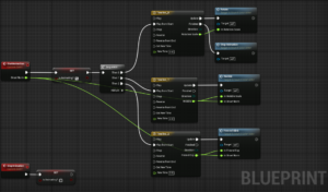
The project “Audio Detection” was part of the M.A. Intermedia Design, at Trier University of Applied Sciences, as an external project. The aim of the project is to combine understanding and skills from the three areas of design, sound and computer science and to work out a verifiable end result. The basic functionality of the developed application is to play and analyze any songs of a user and a visual scene, which adapts dynamically and in real time according to the results of the analysis, without the user having to give further input. However, if the user wants to adjust some settings that serve the application as a kind of frame, he can do so via an additional interface. So-called “onsets” are determined by a recognition algorithm in conjunction with Fast Fourier Transformations and ultimately serve as an event to control visual effects. The project was implemented in the Unreal Engine 4.18, basic audio analysis capabilities in C ++ and all the complementary features in the engine’s own blueprint system. To further enhance performance for real time usage, the algorithm is supported by Nvidia’s CUDA gpu accelerated FFT libraries.
Definition
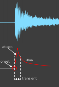
Onset: A moment marking the beginning of a transient or note.
Transient: Short interval during which the signal behaves in a relatively unpredictable way.
Attack: The time interval in which the envelope of the amplitude increases.
Method
Onset Detection Function The basic operation of the Onset Detection Function consists of analyzing a “subsampled” version of the original audio signal. As described in more detail later, the audio signal is divided into consecutive frames consisting of a fixed number of samples. These frames overlap at a certain percentage, the Hop Size. Each result of an ODF or a frame consists of one value. Since onset positions are typically described as the starting point of a transient, it can be said that onset tracking reflects the search for the parts of a signal that are relatively unpredictable (see transient definition). The result of the ODF is given below to a peak-detection algorithm, which determines whether the ODF value belongs to a “real” onset. Peak detection Following the ODF, the detection follows so-called peaks. If the ODF value is above a certain limit, this is localized as a peak at the associated sample position. While the actual selection of the onsets and the finding of a suitable limit value will be explained later, the real-time aspect of the method used should be discussed here. To process a real-time stream of ODF values, the first step in peak detection must be to examine the current values for local maxima. For this, the current ODF value must be compared with the two adjacent (past and future) values. Since the algorithm can not possibly look to the future due to the real-time aspect, both the current and the past ODF value must be stored and waited until the calculation of the next value until this comparison can be carried out. This creates a delay in peak detection. The delay is described by the sample number of the mentioned frames and the sample rate of the original signal, as follows:
As an example, with a FrameSize of 1024 samples and a Sample Rate of 44100 Hz, a delay of approximately:
Limit Calculation
As mentioned in the last section, the ODF results are filtered by a threshold. Only those values that exceed this limit are selected as “real” onsets. Audio signals can quickly take on a complex form, so a fixed limit that does not change will produce bad results when it comes to recognizing onsets of different notes and instruments. Fast varying amplitudes and instruments with, for example, long attack time would produce false onsets. Therefore, a dynamic, “wandering” limit is calculated for the application developed here:
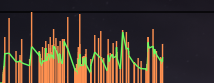
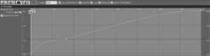
Here, λ and α are weightings for the median or mean, respectively, O [m_n] represents the m-many past ODF values at the n-th frame. N plays a less central role in the limit calculation and in turn, consists of v, the largest peak that has been found so far multiplied by w, a weighting. For a real-time use of the limit, it is recommended to either set the weight w equal to 0 or adjust it at regular intervals to detect changes in the dynamic level of an audio signal. Figure 2 shows the graph of the found onset values (orange) and the corresponding limit value (green), with m = 10, λ = 1, α = 1 and w = 0:
Spectral Difference ODF
There are several different techniques for detecting onsets, which treat the audio signal fundamentally different. One technique that has been very useful in the past is the spectral difference method. Not only can onsets be detected in polyphonic signals, notes playing at the same time, but also instruments that have no percussive character, such as a violin. The spectral difference ODF is calculated by examining changes between the frames in the Short Time Fourier Transform, i.e. in the frequency range of the signal. The Fourier transformation of the nth frame, which is additionally processed with a Hann window function w (m), is given by:
X (k, n) is the kth ‘frequency block’ of the nth frame. The Fourier transform often causes a so-called leak effect, which arises because a continuous signal is divided into finite frequency blocks. The mentioned Hann window function w (m) is here an appropriate method to weight the sampling of the signal and to “fade in and out” in the window area.
An onset usually produces a sudden change in the frequency range of an audio signal, so changes in the average of the spectral difference will often point to an onset. Therefore, the Spectral Difference ODF is generated by summing the spectral difference across all frequency blocks in a frame and is given by:
Linear Prediction
The ODF described so far attempts to distinguish between transient and steady-state regions by making predictions based on information from the current frame and two previous frames. In this section, in a final step, the algorithm is to be supplemented in such a way that the predictions become more accurate. For this the method of linear prediction is introduced. Instead of calculating predictions with only one or two frames, any number of pre-processed frames are used which, together with the LP, give a more accurate estimate. The ODF value is then the absolute difference between the measurements for the current frame and the LP forecasts. The result of the ODF is therefore low, if the LP prediction is accurate and higher in regions that are less predictable, ie where onset occurs. In the LP model, the current sample x (n) is estimated by a weighted combination of past values. The predicted value,
, is determined by FIR filtering as follows:
where p is the order of how many past frames are considered of the LP model and a_k are the coefficients of the prediction. The next step is the calculation of these coefficients. In the literature, the so-called Burg algorithm is used for this, but at this point the precise functioning of the algorithm should be dispensed with in order to provide a deeper insight into the visual implementation of the project.
Spectral Difference and Linear Prediction
In the final step, the linear prediction model is combined with the spectral difference ODF. The spectral difference ODF is formed by the absolute value of the difference in magnitudes of surrounding frequency blocks. This difference can also be seen as a prediction error, because the calculated magnitudes should remain constant as long as the signal does not change decisively. As a reminder, the ODF result is small when the progressive signal changes little and high in transient regions. In the spectral difference ODF with linear prediction (ODF_SDLP), the predicted magnitude value of the k-many frequency blocks in frame n is calculated by using the magnitudes of the corresponding blocks from the previous p frames to calculate the p-many LP coefficients to find. With these coefficients the magnitudes are filtered according to the LP model. So the coefficients of the predicted magnitudes are found by applying the Burg algorithm to the sequence
Let P_SD (k, n) be the predicted spectral difference for block k in frame n, then:
Although this adds significantly more computations per frame, the algorithm can still accommodate real-time needs. How much the LP model influences the effort of the calculations depends on how high the order p of the model is chosen.
The basic goal of the visualization for this project was to illustrate the results of the underlying algorithm to the user on an artistic basis. The previously explained onsets serve as events to control visual effects.
Color Mapping
All reactive elements of the visualization are colored on a dynamic basis according to their defined frequency range. This process uses a combination of the maximum hertz and amplitude values and the average of the amplitude values of the actor’s own frequency range of the current detection cycle. These values are entered in the HSV (Hue-Saturation-Value) range with min. and max. restrictions and then passed as RGB (Red-Green-Blue) value to the shader of the Actors.
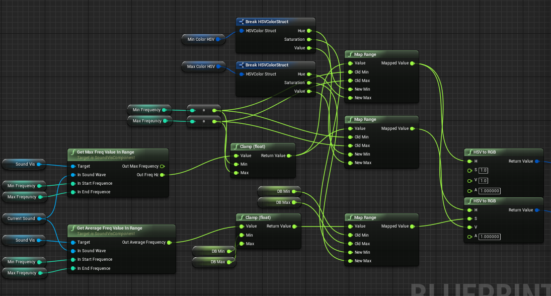
The frequency (Hz) with the maximum amplitude of the range, determines here the Hue value, which color the Actor assumes, the maximum amplitude value the Value value, thus how strongly the Actor shines and the average of all amplitudes in the range, the Saturation Value, the saturation of the color.
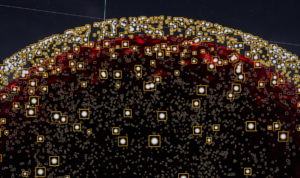
Sphere Actor
The real-time “walk-through” scene consists of several elements that together make up the visual realization of the project. At the center is the sphere actor: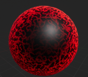
The appearance of the Sphere Actor is described in addition to the general color mapping, by three modes of operation:
1. Fresnel Blink effect: The actor responds to a found onset in which he blinks on. This flashing is described by a Fresnel function. By normalizing the onset value to a 0-1 range, it can be used to calculate the exponent of the Fresnel function in the corresponding shader
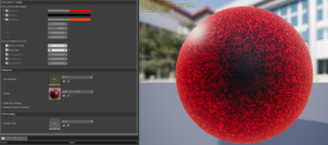
2. wobble effect: The “wobble” effect shows how the individual vertices of the 3D sphere model move when an onset occurs. How strong this effect is is scaled with the normalized onset value.
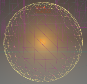
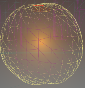
3. Rotation effect: In addition to the wobble effect mentioned above, the Sphere Actor will be rotated by a certain amount every time it is turned on, boosting the wobble effect and adding more dynamics to the movement. In addition, the rotation moves the vertices of the sphere over the noise texture that is in Worldspace (ie the texture is not mapped to the model’s local UV coordinates and is independent of them), giving the viewer the impression that as if small waves were running over the sphere as soon as an onset occurs.
Each of these effects is animated via an individual, time-dependent graph to set an appropriate duration and a non-linear behavior:
Particles
As a shell, the Sphere Actor surrounds a particle system in the form of a bubble. These particles respond to found onsets by moving away from the sphere and then pulling back together.
The animation of the particles works via World Position Offset and is calculated with a time variable in conjunction with a sine function, so that the movement of the particles can be efficiently calculated and yet are smooth. As a local starting point for this movement, serves an “Attraction Point”, a point from which the particles drift away and then move back to. Thus, a kind of artificial physical force is visualized. How much the particles move away from this point is controlled by the current, normalized onset value.
The rest of the scene effects are more or less set up in the same way.
Conclusion
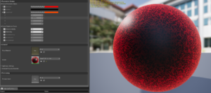
In conclusion, it can be said that the original intention of analyzing an audio track and visually presenting these results has been achieved. The visual representation may be customized for future use as long as it is based on the results of the onset detection or the frequency data of the audio track. Through the implemented interface, the user has enough options to adjust the scene according to his color ideas.